Why Image Enhancement
In the realm of Python and AI, image enhancement is especially crucial.During the process of generating, transmitting or transforming an image, it is affected by a number of factors such as light source, imaging system, and channel bandwidth and noise, which may result in degradation of quality such as low contrast, insufficient dynamic range, loss of clarity, and the inclusion of significant noise. Therefore, image enhancement is required. This is a field where Python and AI technologies are increasingly being applied.
Definition of Image Enhancement
Image enhancement is to improve the quality of an image for some application purpose, and the result of the processing is more suitable for human visual characteristics or machine recognition systems.
Enhancement does not increase the information of the original image, but only improves the ability to recognize certain information, and such processing may cause partial loss of other information. Python and AI techniques contribute to achieving this goal effectively.
Methods of image enhancement
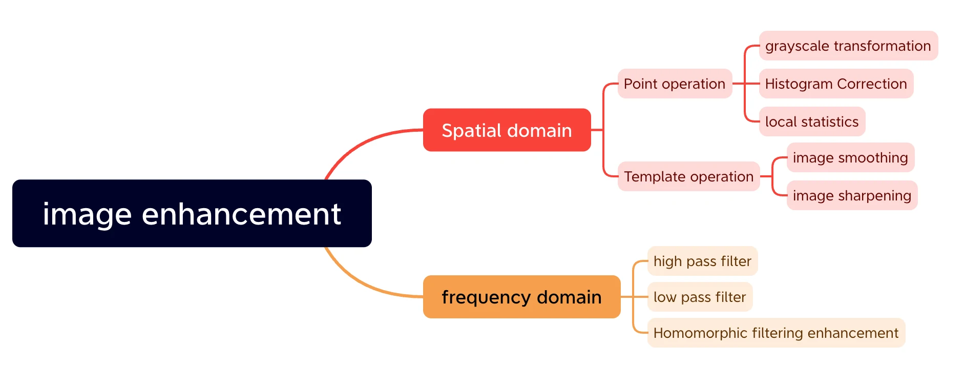
1.Image enhancement methods can be categorized into spatial domain methods and frequency domain methods according to the domain of action. This method can be effectively implemented using Python and AI for upscaling the image quality.
Spatial domain method refers to the image spatial domain directly on the pixel gray value operation processing, commonly used gray scale transformation, histogram correction, template convolution, pseudo-color processing, etc..
Frequency domain method is to enhance the transformed value of the image in some kind of transform domain of the image, and then obtain the enhanced image by inverse transformation, which is an indirect processing method. AI algorithms can also be used for these frequency domain methods.
2. According to the analysis of the frequency characteristics of the image, it is generally believed that the contrast and dynamic range of the entire image depends on the image information
The contrast and dynamic range of the whole image depend on the low-frequency part of the image information (referring to the overall image), while the edge contour and local details in the image depend on the high-frequency part. Therefore, two-dimensional digital filtering methods are used for image processing, such as
High-pass filters are used, which help to emphasize the edge contours and detailed parts of the image.
Low-pass filters are used to smooth the image and reduce noise.
3. Image enhancement methods can be divided into smoothing and sharpening according to the purpose and effect of processing. Python and AI algorithms can help in the effective implementation of these methods for image upscaling
Smoothing has a blurring effect on the image, making the image transition natural and soft, suppressing noise; based on the frequency characteristics of the image from the frequency point of view to understand, smoothing is to maintain or strengthen the low-frequency components of the image, weakening or eliminating the high-frequency components of the image.
Sharpening can be seen as the inverse operation of smoothing, the effect and purpose is to highlight the details, so that the image outline is clear, contrast; from the perspective of frequency domain processing, sharpening is to enhance the high-frequency components of the image.
These methods are based on Python and AI technologies.Next, I introduce 12 ai upscaling methods via python
12 python ai upscaling methods
Here, we introduce 12 AI-driven upscaling methods implemented in Python.”
1.Contrast and brightness enhancement
Usage scenario: bright spot (white spot) detection for dark (black) backgrounds
Realization,This enhancement can be automated using Python and AI:
void adjust(const cv::Mat &src, cv::Mat &dst, const float brightness, const float contrast)
{
	double B = brightness / 255.;
   	double c = contrast / 255.;
	double k = tan((45 + 44 * c) / 180 * M_PI);
	double alpha = k;
	double beta = 127.5 * (1 + B) - k * 127.5 * (1 - B);
	src.convertTo(dst, -1, alpha, beta);
}
2.Histogram equalization
Histogram equalization is a whole image mapping, and will not be mapped locally to certain regions, for those parts of the region is dark or light image is not applicable. At the same time, histogram equalization reduces the gray level of the image, causing some details of the image to disappear. Histogram equalization can be effectively performed using Python libraries.
It is more suitable for an overall dark or light image. It can make the gray value of the whole image evenly distributed in the whole dynamic range [0,255], so as to increase the contrast of the image.
1).Customized cumulative frequency equalization method:
Steps:
- Count the number of pixels per gray value in the image
- Calculate the frequency of each gray value pixel and calculate the cumulative frequency
- Map the image and the gray value of the image = original gray value of the image * cumulative frequency
Single channel:
bool MyEqualizeHist(Mat gray, Mat & result)
{
//Count the number of pixel values from 0 to 255
map<int, int>mp;
for (int i = 0; i < gray.rows; i++)
{
uchar* ptr = gray.data + i * gray.cols;
for (int j = 0; j < gray.cols; j++)
{
int value = ptr[j];
mp[value]++;
}
}
//Count the frequency of 0~255 pixel values, and calculate the counting frequency
map<int, double> valuePro;
int sum = gray.cols*gray.rows;
double sumPro = 0;
for (int i = 0; i < 256; i++)
{
sumPro += 1.0*mp[i] / sum;
valuePro[i] = sumPro;
}
//Convert based on cumulative frequency
for (int i = 0; i < gray.rows; i++)
{
uchar* ptr1 = gray.data + i*gray.cols;
for (int j = 0; j < gray.cols; j++) {
int value = ptr1[j];
double p = valuePro[value];
result.at<uchar>(i, j) = p*value;
}
}
return true;
}
Multi-channel (RGB):
void MyEqualizeHistRgb(Mat& image)
{
	Mat imageRGB[3];
	split(image, imageRGB);
	for (int i = 0; i < 3; i++)
	{
		MyEqualizeHist(imageRGB[i], imageRGB[i]);
	}
	merge(imageRGB, 3, image);

	imshow("result", image);
}
2).opencv comes with equalizeHist():
equalizeHist(Mat src, Mat dst).
Steps:
- Calculate the histogram H of the input image (8-bit);
- Normalize the histogram H so that the histogram bins sum to 255;
- Calculate the integral of the histogram; H′i=∑ 0≤j<i H(j);
- Transform the image using H′ as a look-up table (look-uptable), the transformation formula for specific pixel values is: dst(x,y)=H”(src(x,y))
This algorithm normalizes the brightness and increases the contrast of the image,the result will be different from the customized one.
3).Adaptive local histogram equalization
Local histogram process:
- Set a template (rectangular neighborhood) of a certain size and move it along the image pixel by pixel;
- For each pixel position, calculate the histogram of the template region, and perform histogram equalization or histogram matching transformation on this local region, and the transformation result is only used for the gray value correction of the center pixel point of the template region;
- The template (neighborhood) moves row by row and column by column in the image, traverses all pixel points, and completes the local histogram processing of the whole image.python and AI make it easier to adapt histograms locally for upscaling.
c++ code:
//C++
cvtColor(img,gray,COLOR_BGR2GRAY);
Ptr<CLAHE> clahe = createCLAHE();
clahe->apply(gray, dst);
Python code:
//python
clahe = cv2.createCLAHE(clipLimit=2.0, tileGridSize=(4,4))  # Create CLAHE object
imgLocalEqu = clahe.apply(img)  # Adaptive local histogram equalization
titleGridSize: template (neighborhood) size for local histogram equalization, optional, default (8,8)
clipLimit: threshold for color contrast, optional, default 8
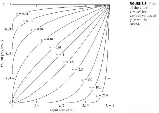
3.Exponential transformation enhancement
Exponential transformation (Power-Law) formula: S = c * R ^ r, through a reasonable choice of c and r can be compressed grayscale range, the algorithm to c = 1.0/255.0, r = 2 to achieve.
Tested with a darker image, the actual effect is darker. Consistent with the formula’s reasoning, the actual pixel value is replaced with the smaller value from the lookup table.
Custom index enhancement algorithm:
void Enhance::ExpEnhance(IplImage* img, IplImage* dst)
{
    // Since oldPixel:[1,256], you can save a lookup table first
    uchar lut[256] ={0};

    double temp = 1.0/255.0;

    for ( int i =0; i<255; i++)
    {
        lut[i] = (uchar)(temp*i*i+0.5);
    }

    for( int row =0; row <img->height; row++)
    {
        uchar *data = (uchar*)img->imageData+ row* img->widthStep;
        uchar *dstData = (uchar*)dst->imageData+ row* dst->widthStep;

        for ( int col = 0; col<img->width; col++)
        {
            for( int k=0; k<img->nChannels; k++)
            {
                uchar t1 = data[col*img->nChannels+k];
                dstData[col*img->nChannels+k] = lut[t1];
            }
        }
    }
}

//  OpenCV versions before 2.1 used the IplImage* data structure to represent images, and versions after 2.1 used the image container Mat to store them.
//	Mat dstImage = cvarrToMat(&dst1); // Convert IplImage format to Mat format
// 	IplImage dst1= (IplImage)(dst);// Convert Mat type image to IplImage

// The following is the original version using Mat.

void Enhance::ExpEnhance(Mat & img,double c, int r)
{
    if(img.channels() != 1)
    {
        cvtColor(img,img,COLOR_BGR2GRAY);
    }

    uchar lut[256] ={0};
    for ( int i =0; i<255; i++)
    {
        lut[i] = (uchar)( c * pow(i,r) +0.5);
        cout << c*i*i+0.5<<endl;
    }

    for(int i = 0;i < img.rows; i++)
    {
        for(int j = 0;j < img.cols; j++)
        {
            int pv = img.at<uchar>(i,j);
            img.at<uchar>(i,j) = lut[pv];
        }
    }
}
Note:Some blogs use expf(n) to calculate the nth power of e. Personally, I think it is wrong. expf(100) is already inf infinity. Implemented in Python, AI algorithms can further optimize exponential transformation.
srcmat.at<uchar>(i, j) = (unsigned char)(255.0 *(expf(srcmat.at<uchar>(i, j) - low_bound) / expf(up_bound - low_bound))); 4. Gamma enhancement
Special exponential enhancement, Gamma correction based on power transformation is a very important nonlinear transformation in image processing, it is the opposite of the logarithmic transformation, it is the gray value of the input image for the exponential transformation, which corrects the deviation in brightness. Python and AI methods provide more options for gamma correction and enhancement. Usually, Gamma correction is used to expand the details of dark tones. Generally speaking, when the value of Gamma correction is greater than 1, the highlights of the image are compressed and the dark tones are expanded; when the value of Gamma correction is less than 1, on the contrary, the highlights of the image are expanded and the dark tones are compressed.
output = L^γ
- When γ is less than 1, the low grayscale interval is stretched and the high grayscale interval is compressed;
- When γ is greater than 1, the low grayscale interval is compressed and the high grayscale interval is stretched;
- When γ is equal to 1, it simplifies to a constant transform.
1. Fixed cubic enhancement:
void Enhance::gammaEhance(Mat& image)
{
	Mat imageGamma(image.size(), CV_32FC3);
	for (int i = 0; i < image.rows; i++)
	{
		for (int j = 0; j < image.cols; j++)
		{
			imageGamma.at<Vec3f>(i, j)[0] = (image.at<Vec3b>(i, j)[0])*(image.at<Vec3b>(i, j)[0])*(image.at<Vec3b>(i, j)[0]);
			imageGamma.at<Vec3f>(i, j)[1] = (image.at<Vec3b>(i, j)[1])*(image.at<Vec3b>(i, j)[1])*(image.at<Vec3b>(i, j)[1]);
			imageGamma.at<Vec3f>(i, j)[2] = (image.at<Vec3b>(i, j)[2])*(image.at<Vec3b>(i, j)[2])*(image.at<Vec3b>(i, j)[2]);
		}
	}
	//Normalized to 0~255
	normalize(imageGamma, imageGamma, 0, 255, CV_MINMAX);
	//Convert to 8bit image display
	convertScaleAbs(imageGamma, imageGamma);
	imshow("gammacubic enhancement", imageGamma);
}
2. Custom coefficient enhancement:
Mat Enhance::gammaWithParameter(Mat &img, float parameter)
{
	//Create lookup table file LUT
	unsigned char LUT[256];
	for (int i = 0; i < 256; i++)
	{
		//Gamma transform definition
		LUT[i] = saturate_cast<uchar>(pow((float)(i / 255.0), parameter)*255.0f);
	}
	Mat dstImage = img.clone();
	//When the input image is a single channel, Gamma transformation is performed directly
	if (img.channels() == 1)
	{
		MatIterator_<uchar>iterator = dstImage.begin<uchar>();
		MatIterator_<uchar>iteratorEnd = dstImage.end<uchar>();
		for (; iterator != iteratorEnd; iterator++)
			*iterator = LUT[(*iterator)];
	}
	else
	{
		//When the input channel is 3 channels, each channel needs to be transformed separately
		MatIterator_<Vec3b>iterator = dstImage.begin<Vec3b>();
		MatIterator_<Vec3b>iteratorEnd = dstImage.end<Vec3b>();
		//Conversion by lookup table
		for (; iterator!=iteratorEnd; iterator++)
		{
			(*iterator)[0] = LUT[((*iterator)[0])];
			(*iterator)[1] = LUT[((*iterator)[1])];
			(*iterator)[2] = LUT[((*iterator)[2])];
		}
	}
	return dstImage;
}
5.Log conversion enhancement
Effective. Test transparent items blurred boundary enhancement after obtaining good results.
Logarithmic transformation can expand the low gray value and compress the high gray level value, so that the gray level distribution of the image is more in line with the visual characteristics of the human eye.
After proper processing, the contrast of low gray areas in the original image will be increased and dark details will be enhanced.python libraries often have built-in functions for logarithmic transformation, useful in AI upscaling.
The logarithmic transformation formula is:
y = log(1+x)/b
where b is a constant used to control the degree of curvature of the curve, where the smaller b is the closer it is to the y-axis and the larger b is the closer it is to the x-axis. The x in the expression is the pixel value in the original image and y is the transformed pixel value.
Realization:
void logEhance(Mat& image)
{
	Mat imageLog(image.size(), CV_32FC3);

	for (int i = 0; i < image.rows; i++)
	{
		for (int j = 0; j < image.cols; j++)
		{
			imageLog.at<Vec3f>(i, j)[0] = log(1 + image.at<Vec3b>(i, j)[0]);
			imageLog.at<Vec3f>(i, j)[1] = log(1 + image.at<Vec3b>(i, j)[1]);
			imageLog.at<Vec3f>(i, j)[2] = log(1 + image.at<Vec3b>(i, j)[2]);
		}
	}
	//Normalized to 0~255
	normalize(imageLog, imageLog, 0, 255, CV_MINMAX);
	//Convert to 8bit image display
	convertScaleAbs(imageLog, image);
	//imshow("Soure", image);
	imshow("Log", image);

}
6.Laplace Ehance enhancement
Has a sharpening effect, more sensitive to noise, need to do the smoothing process first.
Used to improve the blurring due to diffusion effect is particularly effective, because it is consistent with the model of downscaling. Diffusion effect is a phenomenon that often occurs in the imaging process.
The Laplacian operator is generally not used in its original form for edge detection because, as a second-order derivative, the Laplacian operator has an unacceptable sensitivity to noise; at the same time, its magnitude produces an arithmetic edge, which is an undesired result of complex segmentation; and lastly, the Laplacian operator does not detect the direction of the edge. AI algorithms can mitigate the noise sensitivity of the Laplacian operator.
Realization:
void Enhance::laplaceEhance(Mat& image)
{
	Mat imageEnhance;
	Mat kernel = (Mat_<float>(3, 3) << 0, -1, 0, 0, 5, 0, 0, -1, 0);

    //A variety of convolution kernels are available.

    //Mat kernel = (Mat_<float>(3, 3) << 0, 1, 0, 1, -4, 1, 0, 1, 0);
    //Mat kernel = (Mat_<float>(3, 3) << 0, -1, 0, -1, 4, -1, 0, -1, 0);
    //Mat kernel = (Mat_<float>(3, 3) << 0, 1, 0, 1, 3, 1, 0, 1, 0);
    //Mat kernel = (Mat_<float>(3, 3) << 0, -1, 0, -1, 5, -1, 0, -1, 0);

	filter2D(image, imageEnhance, CV_8UC3, kernel);
	imshow("laplaceEhance", imageEnhance);
}
7.Linear transformation
There’s not much to say, it’s just a straightforward linear transformation. Linear transformations are straightforward to implement in Python for upscaling purposes.
y = kx+b.
Realization:
Mat Enhance::linearTransformation(Mat img, const float k, const float b)
{
    Mat dst = img.clone();
    for(int i=0; i<img.rows; i++)
    {
        for(int j=0; j<img.cols; j++)
        {
            for(int c=0; c<3; c++)
            {
				float x =img.at<Vec3b>(i, j)[c];
				dst.at<Vec3b>(i, j)[c] = saturate_cast<uchar>(k* x + b);            }
        }
    }
	return dst;
}
8.Segmented linear stretching algorithm
A commonly used algorithm in image grayscale transformation, which also has a corresponding function in the commercial image editing software Photoshop. Segmented linear stretching is mainly used to improve image contrast, highlighting the image details. Python and AI are effective tools for segmented linear stretching, which improves image contrast.
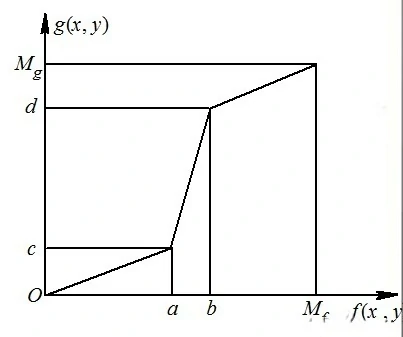
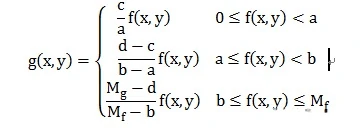
Customized enhancement, weakened pixel intervals:
void Enhance::PiecewiseLinearTrans(cv::Mat& matInput, float x1, float x2, float y1, float y2)
{
	//Calculate straight line parameters
	//L1
	float K1 = y1 / x1;
	//L2
	float K2 = (y2 - y1) / (x2 - x1);
	float C2 = y1 - K2 * x1;
	//L3
	float K3 = (255.0f - y2) / (255.0f - x2);
	float C3 = 255.0f - K3 * 255.0f;

	//build lookup table
    uchar LUT[256] ={0};
	for (int m = 0; m < 256; m++)
	{
		if (m < x1)
		{
			LUT[m] = m * K1;
		}
		else if (m > x2)
		{
			LUT[m] = m * K3 + C3;
		}
		else
		{
			LUT[m] = m * K2 + C2;
		}
	}
	//grayscale map
	for (int j = 0; j < matInput.rows; j++)
	{
		for (int  i = 0; i < matInput.cols; i++)
		{
			//Lookup table gamma transformation
            int x = matInput.at<uchar>(j,i);
            matInput.at<uchar>(j,i) = LUT[x];
		}
	}
}
9.Gray level layering
The simplest example is the commonly used opencv binarization algorithm: thresh, inRange can be. Python libraries like OpenCV offer functions for gray level layering in AI upscaling.
10.Overexposure to the image inverse
Just do a 255-x operation on the value. This is easily achieved using Python code and can be part of an AI upscaling pipeline.
Realization:
void ExporeOver(IplImage* img, IplImage* dst)
{
	for( int row =0; row height; row++)
	{
		uchar *data = (uchar*)img->imageData+ row* img->widthStep;
		uchar *dstData = (uchar*)dst->imageData+ row* dst->widthStep;
		for ( int col = 0; colwidth; col++)
		{
			for( int k=0; knChannels; k++)
			{
				uchar t1 = data[col*img->nChannels+k];
				uchar t2 = 255 - t1;
				dstData[col*img->nChannels+k] = min(t1,t2);
			}
		}
	}
}
11.High contrast retention
High-contrast retention is mainly the image of the color, dark and light contrast between the two parts of the junction retained, such as the image of a person and a stone, then the outline of the stone and the outline of the line of the person and the face, clothing, and other obvious lines of the place will be changed to be retained, the child of the other large-scale changes in dark and dark without obvious changes in the place of generation of medium-gray. python and AI algorithms make high-contrast retention more accurate.
The expression form is:
dst = r*(img – Blur(img)).
Realization:
Mat HighPass(Mat img)
{
	Mat temp;
	GaussianBlur(img, temp,Size(7,7),1.6,1.6);

	int r=3;
	Mat diff = img + r*(img-temp); //High contrast preservation algorithm
	return diff;
}
12.Masaic algorithm (mosaic)
In the daily sometimes confidential or other needs to mosaic the image, the following algorithm to achieve the image mosaic function (principle: the center pixel to represent the neighboring pixels).
uchar getPixel( IplImage* img, int row, int col, int k)
{
    return ((uchar*)img->imageData + row* img->widthStep)[col*img->nChannels +k];
}

void setPixel( IplImage* img, int row, int col, int k, uchar val)
{
    ((uchar*)img->imageData + row* img->widthStep)[col*img->nChannels +k] = val;
}

//nSize: is the size, odd number
//Replace the value of the neighborhood with the value of the center pixel
void Masic(IplImage* img, IplImage* dst, int nSize)
{
    int offset = (nSize-1)/2;
    for ( int row = offset; row <img->height - offset; row= row+offset)
    {
        for( int col= offset; col<img->width - offset; col = col+offset)
        {
            int val0 = getPixel(img, row, col, 0);
            int val1 = getPixel(img, row, col, 1);
            int val2 = getPixel(img, row, col, 2);
            for ( int m= -offset; m<offset; m++)
            {
                for ( int n=-offset; n<offset; n++)
                {
                    setPixel(dst, row+m, col+n, 0, val0);
                    setPixel(dst, row+m, col+n, 1, val1);
                    setPixel(dst, row+m, col+n, 2, val2);
                }
            }
        }
    }
}
Conclusion
The above many methods in practice sometimes are not used alone, filtering and the combination of each method with each other often achieve better results.
If you have a need for image enhancement, you can also use the tools on our website to realize it!
The use of Python and AI for image upscaling and enhancement is highly effective and offers a range of methods to improve image quality.